Note on Terminology
WithinsemanticGIS, we use the concept of design rationale as a practical tool to help you structure and reflect on your GIS project work. Traditionally, the term is used in software and product design to describe decisions after they have been made (see Wikipedia), we’re adapting it here for you to actively plan, document, and justify your decisions as you proceed. Think of it as a blend between a traditional design rationale and a research design.
Like a research design, your rationale will help you plan your work step by step—defining your problem, identifying key concepts, selecting data, and choosing appropriate analytical methods. At the same time, like a traditional design rationale, you’ll be asked to reflect on your decisions, explain why you made them, and consider possible alternatives. This will strengthen your ability to communicate your work clearly to clients, collaborators, or your future self.
A key purpose of the design rationale is to clearly explain the consequences or artefacts created by different choices. By explicitly documenting the trade-offs and potential impacts of various decisions, the rationale helps avoid unintended consequences and ensures that all stakeholders understand the implications of the project’s design.
Moreover, the design rationale is essential for documentation and feedback. It provides a structured record that can be referenced throughout the project’s lifecycle, making it easier to review decisions, provide feedback, and make adjustments as needed. It also serves as a valuable resource for future projects, offering insights into the decision-making process and the outcomes of past choices.
In alignment with the concept developed by W.R. Kunz and Horst Rittel, the design rationale in a GIS project provides an argumentation-based structure that supports the collaborative and often complex process of designing geospatial systems. It ensures that decisions are not only recorded but also justified, considering all alternatives and trade-offs, ultimately leading to more robust and well-founded project outcomes.
By maintaining a clear and detailed design rationale, GIS professionals can enhance the transparency, consistency, and effectiveness of their projects, ensuring that the reasoning behind every decision is well-documented and understood.
Example Design Rationale: Identifying Entertainment Zones in Copenhagen
Below is a sample design rationale for a fictive project where the client (in this case, your teacher) has asked for a data-driven identification and visualisation of Copenhagen’s party/entertainment zones. This example follows the four phases outlined above.
2.1 Project scoping
The project task is to identify party/entertainment zones in Copenhagen using data-driven GIS methods. Since the term “party/entertainment zone” is open to interpretation, I have chosen to define it as areas characterised by a high concentration of social, cultural, and nightlife activities. This includes bars, restaurants, music venues, cinemas, and event spaces. I would like to include some seasonality in the investigation since there are some clear summer-related areas, such as public parks and swimming zones.
Entities relevant to this include:
- Point locations of venues (bars, clubs, theatres, etc.)
- Potential locations for informal party activity (Parks, swimming zones)
- Observations of formal and informal party activity.
- Public transportation nodes (metro stations, bus stops)
- Street network data (for walkability analysis relative to public transport)
Example of detail consideration on bars: To make the analysis meaningful, we need to be precise about what we include under each category. For instance, when working with point locations of venues, we must consider how to define a “bar.” Do we include only standalone bars, or do bars inside clubs, theatres, and cinemas count as well? If a bar is only accessible to ticket holders (e.g., in a theatre or amusement park), should it be included? In this project, I have decided to include bars that are publicly accessible, whether they are standalone or part of a larger establishment. Bars within clubs or theatres are only counted if they serve the general public. Bars in amusement gardens with entrance fees are included, as they contribute significantly to the entertainment landscape. Finally, we also need to look at temporality some establishments might only be open at weekends or in the summer period. Careful attention must also be paid to avoid double-counting venues (e.g., not counting a club and its bar as two separate entities unless they function independently).
2.2 Data Modelling
In this case, our ontology of a bare is rather vague and it can match up with bars in at least three alternative datasets:
- The Danish register for firms CVR that use standard NACE codes NACE code 563020 = Beverage serving activities.
This is probably the most reliable dataset, but it might have some bios due to its official purpose for taxation. - Open Street map: the ontology is here based on key and tags in the case of a bar we could use the key amenity with the tag ‘bar’ or ‘pub’ Tag = bar: is used to map a bar: a purpose-built commercial establishment that sells alcoholic drinks to be consumed on the premises. They are characterised by a noisy and vibrant atmosphere, similar to a party. They usually do not sell food to be eaten as a meal. The music is usually loud and you often have to stand. Sometimes it has a dancefloor, but it’s not the main attraction. Tag = bar :A pub or public house is an establishment that sells alcoholic drinks that can be consumed on the premises. Pubs commonly sell food which also can be eaten on the premises. They are characterised by a traditional appearance and a relaxed atmosphere. You can usually sit down and there is usually no loud music to disturb conversation. A pub would be a good location to meet after a day’s mapping for OpenStreetMap.
- Google Maps place API: the term bar is defined as “a physical establishment that serves alcohol, which is categorized by Google Maps based on its business information and reviews” In this case, any of the definitions (DoD) could be used and we can continue to the next phase of sourcing the data
2.3 Data Sourcing and Preparation
The following is an example of the considerations you might make in this case, looking at data for bars.
As mentioned, there are at least three alternatives to source for this data.ther the ontology of bar matches:
- The Danish register for firms CVR that use standard NACE codes (available in English).
- Open Street map: the ontology is here based on tags and values in the case of a bar we could use the tag amenity with the tag (‘bar’, ‘pub’)
- Google Maps place API: I considered using commercial venue data (e.g., Google Places), but decided against it due to licensing restrictions.
Both 1 and 2 are plausible and free, but before deciding on which dataset to use for representing bars, I conducted a quick comparison of available sources:
To acquire OSM data, I used QuickOSM and searched for the tag amenity within the extent of Copenhagen Municipality. Although the initial query included locations outside the municipality boundary, I clipped the resulting layer using the official administrative boundary of Copenhagen. I then filtered the features where amenity was in (‘bar’, ‘pub’), which resulted in 534 potential bar locations.
From the CVR (Danish Central Business Register), I downloaded a list of all active business units (p-enheder) in Copenhagen and filtered them using the NACE code 563020, which corresponds to bars. This gave me 680 businesses, but these lacked spatial coordinates—only address information was available. I joined these with a geocoded address dataset and filtered out those located outside Copenhagen, resulting in 552 mappable bars.
To manage the risk of data loss and ensure a clean workflow, I saved the layers as CVR_bar and OSM_bar, converted both to EPSG:25832 and removed unnecessary attributes. A visual comparison showed better alignment between Google Maps and OSM than between Google Maps and CVR, which influenced my final decision.
Although the CVR data might be more authoritative in terms of business registry, it lacked up-to-date changes and required extensive processing. Based on completeness, alignment, and ease of use, I chose to continue with the OSM dataset. Ideally, I would validate this through field mapping, but time constraints prevented this step.
Other datasets not described in detail:
-
Parks and other leisure areas.
-
Noise complaint records (as a proxy for nightlife activity) Copenhagen noise complaint data, police reports. This might also need some fieldwork.
-
Rejseplanen’s GTFS feed for public transport locations or OSM trafic data
-
Official GeoDanmark or OpenStreetMap street network data for walkability analysis
2.4 Analytical Approach
The problem was deconstructed into a set of GIS operations:
- 1.Venue Density Analysis: I used kernel density estimation on entertainment POIs to identify spatial clusters. In considering how to model the spatial distribution of bars, I evaluated two main options: analyzing counts per cell in a regular grid or applying a kernel density function. While a grid-based approach (e.g., 250x250m cells) offers clarity and ease of interpretation, I found that kernel density estimation better captured the gradual influence of multiple venues on an area’s ambiance. I selected a quartic kernel function with a search radius of 500 meters, based on the assumption that a bar can contribute to the perceived liveliness of an area up to 500 meters away. This distance approximates a 5–7 minute walk and reflects how clusters of venues influence urban atmosphere. A uniform kernel was considered, but the quartic kernel was preferred for its smoother decay of influence with distance, better reflecting the nature of urban entertainment clustering.
Not so-detailed discussion. 2. Noise Hotspot Mapping: Noise complaint points were aggregated by 100x100m grid to reveal concentration areas.
-
Walkability Analysis: A service area analysis was performed around public transport nodes to highlight accessible zones.
-
Zoning Filter: Entertainment clusters were cross-referenced with zoning layers to exclude incompatible land use areas.
These steps were combined in a weighted overlay to generate a final raster surface representing entertainment potential. Alternative approaches were considered (e.g., DBSCAN clustering), but kernel density provided better control over smoothing and visibility.
2.5 Dissemination and Communication
The results are presented in two main formats:
-
An interactive web map (built using QGIS and Leaflet) to allow clients to explore the zones in detail.
-
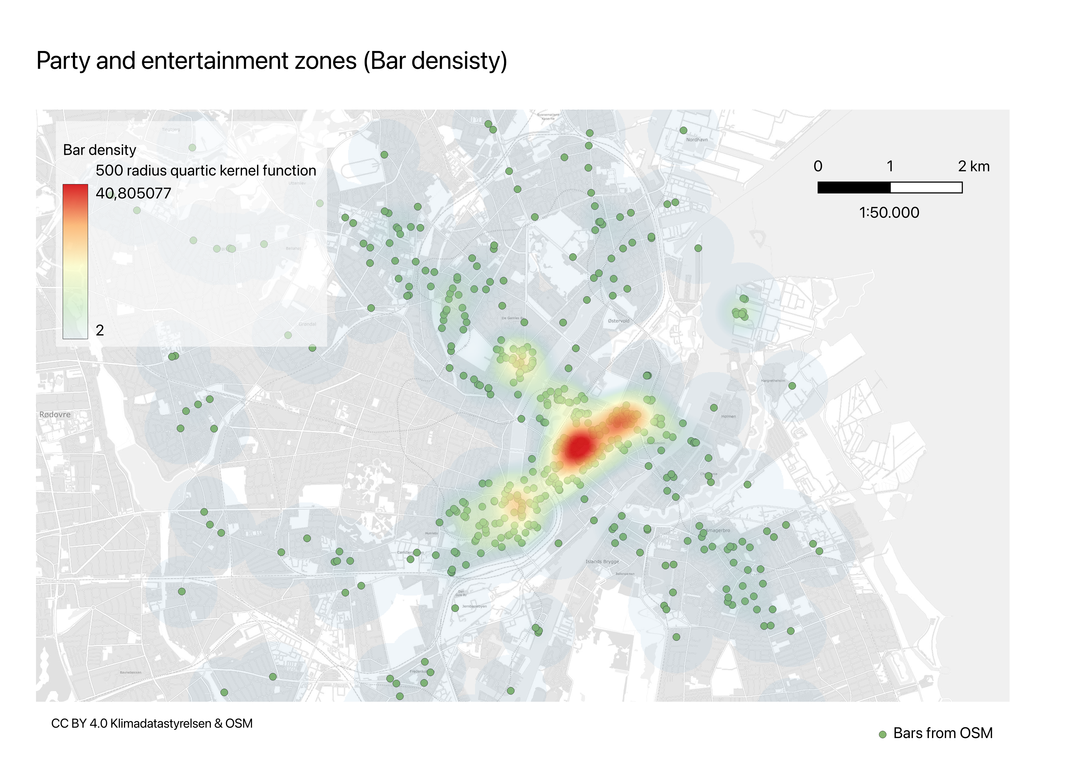
A summary report with static maps and charts tailored to a policymaker audience. One key element of this report is a map showing the result of the venue density analysis. For this map, I chose a light gray background to avoid visual interference with the color gradient used to represent bar density. The density scale runs from blue (indicating low or “boring” levels of activity) to red (indicating a high-intensity party zone).
Summery report map in detail: To enhance interpretability, I decreased the opacity for low-density values so that only significant concentrations are emphasized. A detailed description of the methodology is included directly on the map, stating that it shows bar density based on a 500-meter radius quartic kernel function.
The map is included as an appendix to ensure it can be printed at A4 size like the rest of the report. This choice also allowed me to select a round and readable map scale of 1:5000. Both a scale bar and a numeric ratio (e.g., 1:5000) have been included and placed in the water area outside Copenhagen to avoid covering relevant data.
Finally, a source credit—‘CC BY 4.0 Klimadatastyrelsen & OSM’—has been added to acknowledge the background map and venue data. No additional legend or title was added, as the map is meant to be interpreted in the context of the report’s discussion.