Horisontal flow over a surface

Surface Water Flow

The Core Problem: Determining the paths of water, water-borne sediment, and contaminants through a landscape is a key problem in many applications. All algorithms simulating water flow over a surface are guided by the simple principle that water flows downward in response to gravity. While this is a reasonable start assumption, in a digital model, it has some severe side effects that must be addressed. In the digital model, water flow is typically simulated using a raster data dataset representing elevation (a DTM or DSM), which again is a result of interpolating Lidar data. To a computer, this is just a grid of numbers representing the elevation and the basic rule of water flowing downwards implies water will flow from a cell with a higher value to a neighbouring cell with a lower value. However, there are some basic questions

1. What to do if there is more than one neighbouring cell with values lower than the current cell?
2. What to do if there are no neighbouring cells with lower values ?

Answering Question 1: How Do We Distribute the Flow?

This is the problem of flow partitioning. When the elevation cell under squatting is on a ridge or even on a simple hillside, there is often more than one neighbouring cell with a lower elevation value, water can flow into. Allas, there is no single good solution to how to solve this problem. There are three different common algorithms, all with their own Implication.

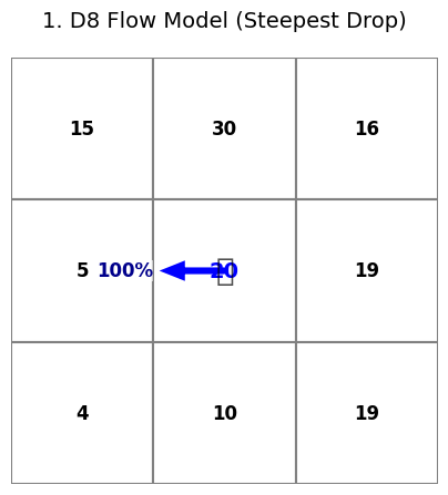
1. The D8 Model (Single Flow Direction)

This is the classic and simplest solution.

• How it works: The algorithm looks at all 8 neighbouring cells and finds the one with the steepest gradient (steepest drop). It then assigns 100% of the flow from the centre cell to that single neighbour.

• The Implication: This model is “deterministic” and computationally fast. However, it’s a poor representation of real-world physics. On a ridge or flat plain, it forces flow into the winner-takes-it-all cell, which does not model divergent flow (water fanning out). It’s best suited for steep, V-shaped valleys where flow is highly convergent. This algorithm tends to concentrate (overestimate) flow in gullies and underestimate the water availability on slopes.

• 

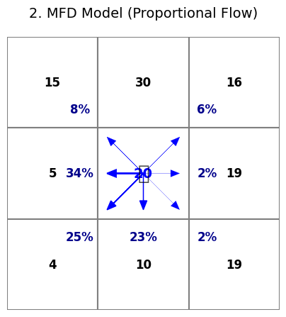
2. The Multiple Flow Direction (MFD) Model

This model was designed to solve the D8 problem.

• How it works: Instead of finding the single steepest cell, this algorithm looks at all neighboring cells that are lower than the center cell. It then partitions the flow among them. The amount of flow each neighbor receives is proportional to its gradient—the steeper the drop, the more flow it gets.

• The Implication: This is much better at modelling divergent flow and how water spreads across a landscape. It’s an excellent choice for modelling how runoff might spread out from a farm field or across a gentle slope. Its weakness is that it can sometimes be too dispersive, “smearing” the flow too much.

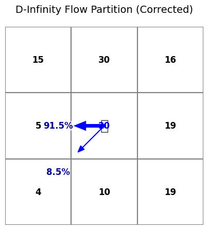
3. The D-Infinity (D$\infty$) Model

This is a more sophisticated, physically realistic model that combines the two previous models.

• How it works: The D-Infinity model differs dramatically from the two other algorithms in that, instead of calculating the slope by comparing the centre points of the grid cells, it creates triangular facets that connect the centre points and calculates the slope based on these facets. For the unconstrained “free flowing” facets, a normal slope is calculatet for that triangle. If the triangle is constrained “not free flowing” a special algorithm is used to calculate the slope see 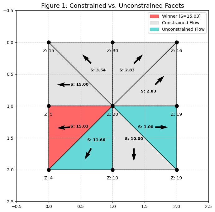The algorithm then splits the flow between the two cells The proportion each cell gets is based on how close the vector angle is to that cell’s center.

• 

• The Implication: This is often the best compromise. It allows for flow to spread (diverge) on ridges and concentrate (converge) in valleys in a way that is less “smeared” than MFD and less “artificial” than D8.

The model you choose is a critical analytical decision. Will severely influence any later calculations within digital hydrology.

Answering Question 2: How to handle tapped water

In a digital hydrological model, water gets trapped if all surrounding cells have higher values than the centre cell. In the real world, this happens all the time and creates puddles. In the real world, these puddles can sometimes grow so large that they overflow. However, in most digital hydrological models there is no such overflow function since they typically do not simulate rain over time but calculate a simple flow. There are three standard solutions to this

1. Increase the elevation of the depressions (low values ) until there are no surrounded cells with higher values. This is by far the most common approach and is called fill
2. Use specialised algorithms that use a path of least resistance, i.e let the water flow on from the point where the barrier is lowest. This wUrnill in many cases result in the same flow pattern as a fill but other properties such as slope is influenced by the fill
3. Burn holes in the bariers. This approach is typically used to handle situations where bridges and other artefacts cross an entire valley and therefore would create a large lake/depression. These situations are typically wrong since water can flow under the bridge or through drainage pipes under roads. In Denamrk ther is a special cocalle hydrological correction layer that contains information on wher to burn holes. It is recommended always tirst to burn holmes

The Flow Accumulation grid—and thus any subsequent analysis like Topographic Wetness Index (TWI)—will look dramatically different depending on whether you chose D8, MFD, or D$\infty$.

An algorithm simulating water flow will stop, or “get trapped,” in any cell that is lower than all its neighbors. We call these cells “sinks.”

A Critical Distinction: Sinks are Features, Not Just Errors The term “hydrologically incorrect” is misleading. It’s not that the data is wrong; it’s that the raw data doesn’t represent the process we want to model. Sinks are often real:

• Landscape Sinks: In the Danish post-glacial landscape, features like “dødishuller” (kettle holes left by melting ice blocks) are true sinks. They are natural retention basins.

• Urban Sinks: In a city (using a DSM), real sinks are everywhere: courtyards, parks with raised curbs, underpasses, or any area designed to hold water.

The Goal: Conditioning the Surface to Model a Process To model connected overland flow (i.e., how water moves across the entire landscape), we must first simulate what happens within these sinks. We do this by “filling” them.

The fill operation simulates a rain event. It fills these sinks with “digital water” up to their “pour point”—the lowest cell on their rim. Once filled, the water “spills” out of this pour point and continues its flow across the landscape.

“Filling” is a Modeling Choice, Not a “Fix” This is the most important step. You are not “fixing errors”; you are setting the parameters of your simulation. This is why many fill tools (like in Whitebox) have a maximum fill depth parameter:

• No max_fill (infinite): This is for a theoretical, macro-scale analysis. You are asking, “What is the total theoretical drainage network if all basins fill and spill?” This is common for regional catchment delineation.

• High max_fill: This models a major storm event (e.g., a 100-year storm). You assume large depressions will fill and connect.

• Low max_fill (e.g., 0.15m): This models a small, specific rain incident. You are simulating curb-level flooding. Water will pond in shallow depressions but might not be deep enough to spill out of larger ones (like a park). This is essential for urban modeling and LAR solutions.

Therefore, “hydrological conditioning” is your first and most critical modeling decision. The parameters you choose define the scientific question you are asking.

• The Goal: We must “condition” the DEM to create a “hydrologically correct” surface. This means ensuring every cell has an uninterrupted downhill path to the edge of the dataset. This conditioned DEM is our “digital twin” of the landscape’s drainage potential

One of the main sources of errors in horological modelling is bridges. The problem is that terrain models often are generated from Lidar scanning of the surface, resulting in the bridge being represented as the surface. In practice, this means that the bridge functions as a dam in the hydrological model. To ensure correct hydrological modelling, it is common to create where bridges are removed.