Visualising multispectral images
Chapter 4 of Remote sensing.
Grey-scale images
A single band is usually shown in shades of grey: the brighter the pixel, the higher its value, and the more radiation the surface reflected in that band. Beyond brightness, a grey-scale image can be read from shape, texture and context (see Image interpretation and classification).
Colour composites
A screen mixes every colour from red, green and blue light. Any three bands can be shown together by assigning one to each of the three colours: an RGB colour composite.
True colour
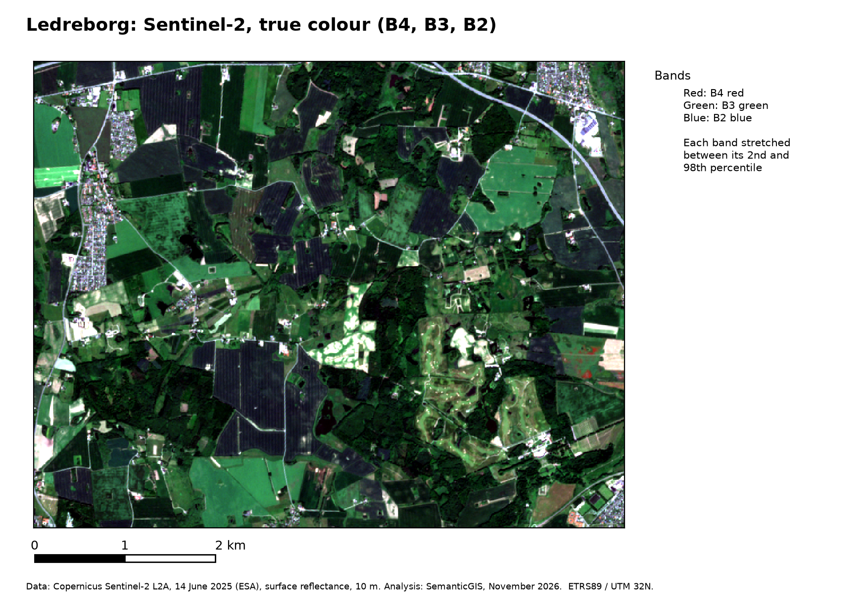
If the red, green and blue bands are shown in red, green and blue, the image looks roughly as the eye would see it. For Sentinel-2: R = B4, G = B3, B = B2.
False colour
Any other assignment is a false colour composite. The most common shows near infrared in red, red in green and green in blue, R = B8, G = B4, B = B3, called colour infrared (CIR). Growing vegetation reflects strongly in the near infrared, so it shows in shades of red that differ with type and condition. Clear water is dark; turbid water, with sediment that reflects red light, is cyan. Bare soil, roads and buildings show as blue, grey or brownish, depending on their material.
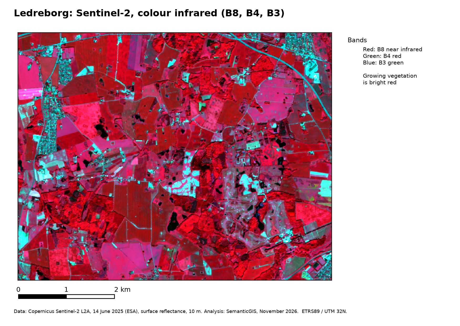
In the colour-infrared image of Ledreborg (14 June 2025) the forests are dark, textured red, the fields smooth red or pink depending on the crop, bare and dry surfaces, roads and buildings cyan to white, and the lakes black. In the true-colour image of the same date nearly all of it is a similar green.
Common band combinations
A composite with a short-wave infrared band, such as R = B12, G = B8A, B = B4, separates moisture and bare soil better. Common combinations, with the Landsat 8 bands they were defined for:
| Purpose | Sentinel-2 (R, G, B) | Landsat 8 |
|---|---|---|
| True colour | B4, B3, B2 | 4, 3, 2 |
| Colour infrared (vegetation) | B8, B4, B3 | 5, 4, 3 |
| False colour (urban) | B12, B11, B4 | 7, 6, 4 |
| Agriculture | B11, B8, B2 | 6, 5, 2 |
| Atmospheric penetration | B12, B11, B8A | 7, 6, 5 |
| Healthy vegetation | B8, B11, B2 | 5, 6, 2 |
| Land and water | B8, B11, B4 | 5, 6, 4 |
| Natural with atmospheric removal | B12, B8, B3 | 7, 5, 3 |
| Short-wave infrared | B12, B8, B4 | 7, 5, 4 |
| Vegetation analysis | B11, B8, B4 | 6, 5, 4 |
A combination is chosen to bring out a contrast that matters for the question: between crops, between wet and dry, between built and bare. It is also a first step towards change detection and classification.
Contrast stretch
A screen shows each colour with values from 0 to 255. Surface reflectance runs from 0 to 1 (0 to 10,000 as stored), but most pixels of a scene use only a small part of that range: vegetation reflects 0.02–0.05 in red. Mapping the full range to 0–255 gives a dark, flat image. A contrast stretch maps only the range that holds most of the values:
- Minimum–maximum: from the lowest to the highest value; a few extreme pixels (clouds, roofs) make the rest dull.
- Cumulative count cut: from, say, the 2nd to the 98th percentile, ignoring the extremes. QGIS uses this by default.
- Mean ± standard deviations: from the mean minus n standard deviations to the mean plus n.
- Gamma: bends the stretch away from a straight line. A gamma below 1 brightens the image, above 1 darkens it.
The histogram of a band, the number of pixels at each value, shows where the values lie before you choose. A dark image has its histogram squeezed into the low end. A stretch only changes the display, never the values used in calculations. Two images stretched separately cannot be compared by their colours.