Soil carbon and land use at Ledreborg — Example

A worked case for the course Environmental Regulation and Management with GIS, Theme 2.2 (carbon storage in land-use systems). Companion: Habitat network at Ledreborg (Example).

At Ledreborg the topsoil holds the most organic carbon where the landscape holds the most nature. The valley system averages 2.2 % SOC in 0–30 cm, the till plain 1.6 %. The difference comes from the wet areas: in wet nature the topsoil holds 6.4 % SOC, in intensive arable land 1.5 %.

Example data

Everything this example uses, frozen as it was used (27 October 2026), so its numbers can be reproduced without API keys: ledreborg_example_data.zip (2.9 MB), a snapshot package. It holds one GeoPackage with the landscapes, protected nature, woodland, hedges and streams; Basemap04 land use and soil organic carbon (0–30 cm) as 10 m rasters with their styles; the Basemap04 class list (codelists/); and snapshot.json and a README with sources, licences and attribution. The same data serve Habitat network at Ledreborg (Example) and Soil carbon and land use at Ledreborg (Example).

1. Spatial Intent

Question: how do land use and soil organic carbon (SOC) differ between the landscapes of the study area, and how does carbon follow land use?

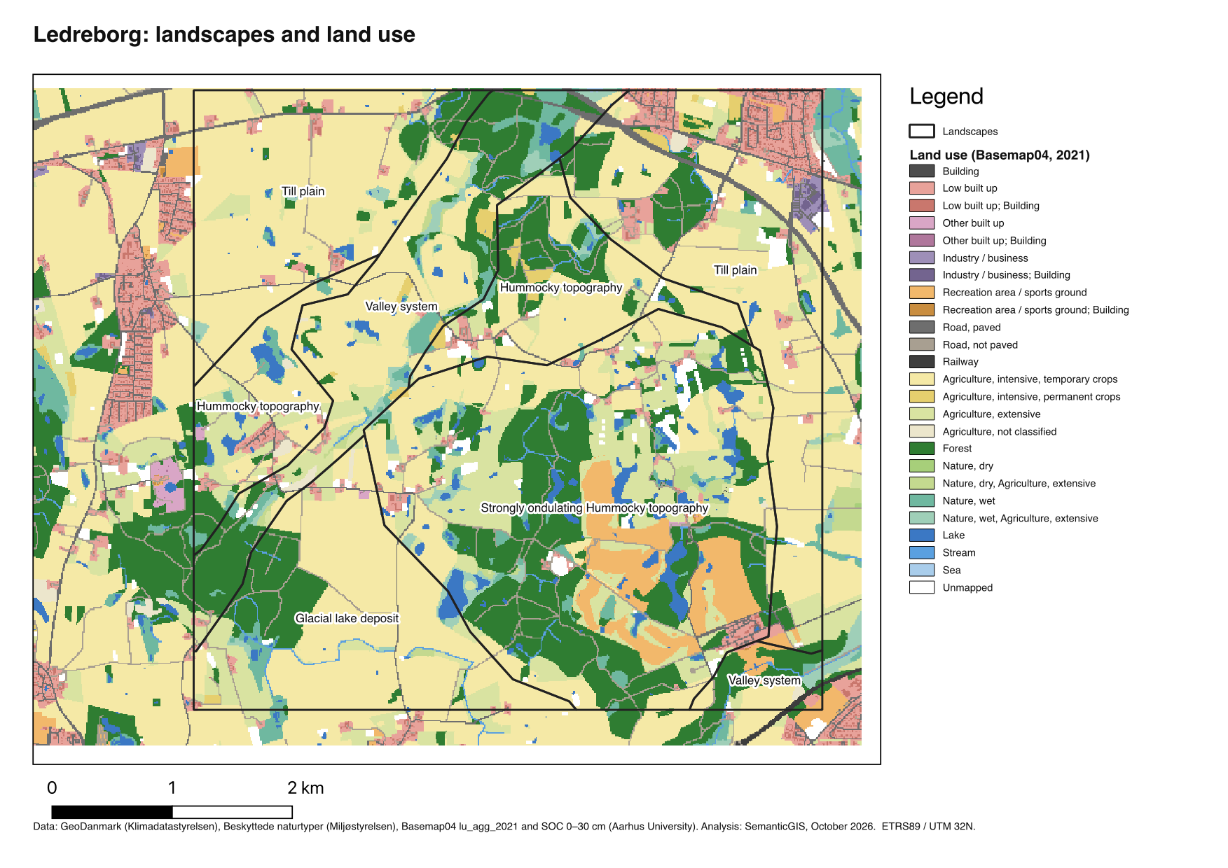
Study area and zones: the five landscape types of the Ledreborg study area (Landscape delineation (Task)).

Theory: photosynthesis takes carbon from the atmosphere into biomass. Part of it ends up in the soil, where microbial activity breaks it down or binds it. How much stays depends on land use (tillage, permanent cover) and on water: in wet soils breakdown is slow, and peat builds up.

2. Auditing the data

Data	Source	What it is	Choices
Land use	Basemap04, lu_agg_2021 (10 m)	35 aggregated classes	legend from the attribute table (lu_agg_2021.qml); classes grouped into ten for the chart
SOC 0–30 cm	Kulstofkort i 10 m opløsning, Aarhus University (10 m)	% organic carbon by mass, modelled from >83,000 samples with Sentinel-1/2 time series and environmental layers	used as a concentration, not a stock; mean and median reported

Known limits: SOC is modelled, with its own error. The model predicts values under lakes and buildings too. 3.4 % of the landscape area has no value. A concentration in % says nothing about tonnes per hectare without bulk density.

3. The Analytical Schema

flowchart LR
  L[Landscape delineation] --> C[Land-use composition per zone]
  L --> Z[Zonal summary of a surface]
  LU[Basemap04 land use] --> C
  SOC[SOC 0–30 cm] --> Z
  LU --> Z

Task	Recipe	Operator families used
Aggregating a categorical raster to zones (Task)	Aggregating a categorical raster to zones (Recipe - QGIS)	Geometry restructuring, Zonal
Aggregating a continuous raster to zones (Task)	Aggregating a continuous raster to zones (Recipe - QGIS)	Geometry restructuring, Zonal

Settings used

• Land use per landscape (Aggregating a categorical raster to zones (Recipe - QGIS)): raster lu_agg_2021.tif (Basemap04, 10 m, 35 classes) with its style lu_agg_2021.qml (English labels; lu_agg_2021_da.qml for Danish), made from the raster’s attribute table. Landscapes dissolved by type; Tabulate area with Report as percent.
• SOC per landscape (Aggregating a continuous raster to zones (Recipe - QGIS)): raster kulstof_kombineeret.tif, SOC 0–30 cm in % by mass, NoData −1. Landscapes dissolved by type; Zonal statistics Count, Mean, Median.
• SOC per land use: Raster layer zonal statistics with lu_agg_2021 as zones; both rasters on the same 10 m grid.

4. Results

Land use

Soil organic carbon

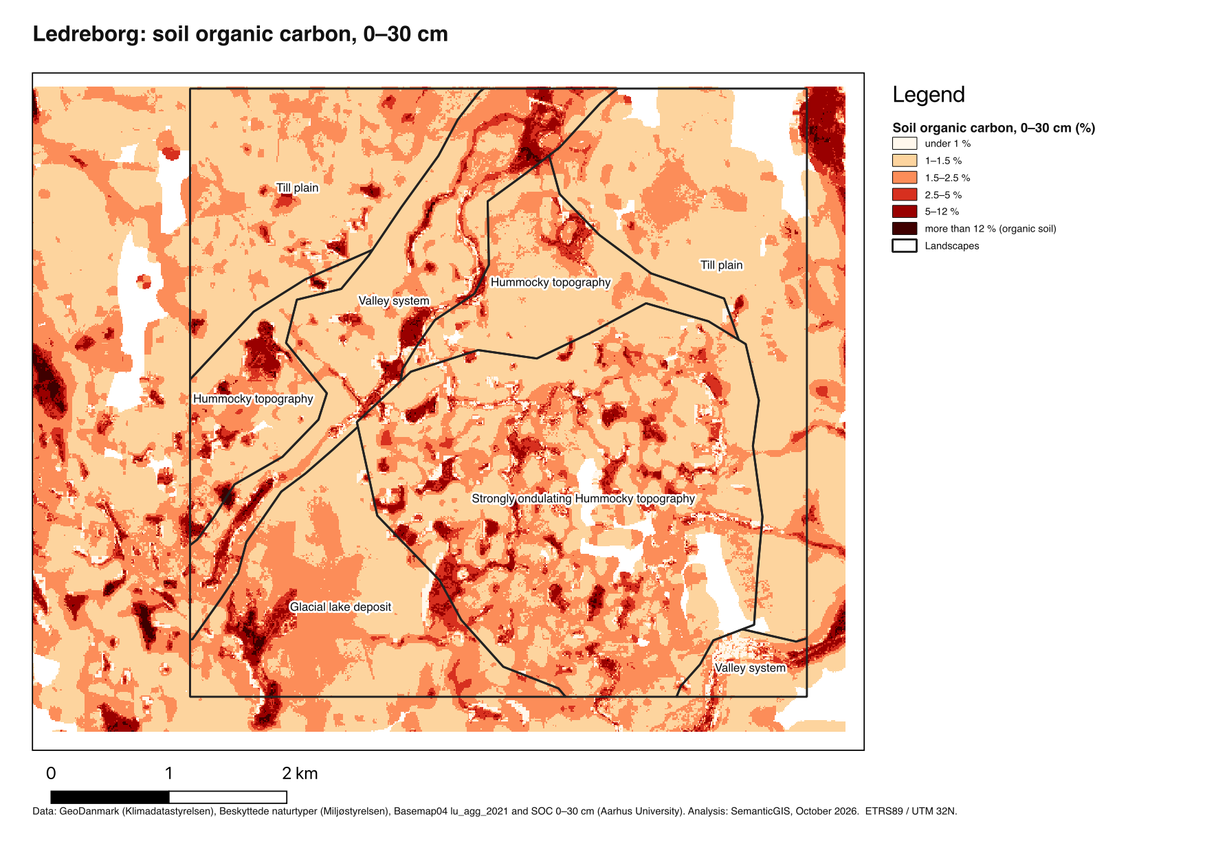
High SOC values follow the valleys and the hollows between the hummocks: the wet areas and former peatland. On the till plain the topsoil is uniformly low.

Land use and SOC per landscape

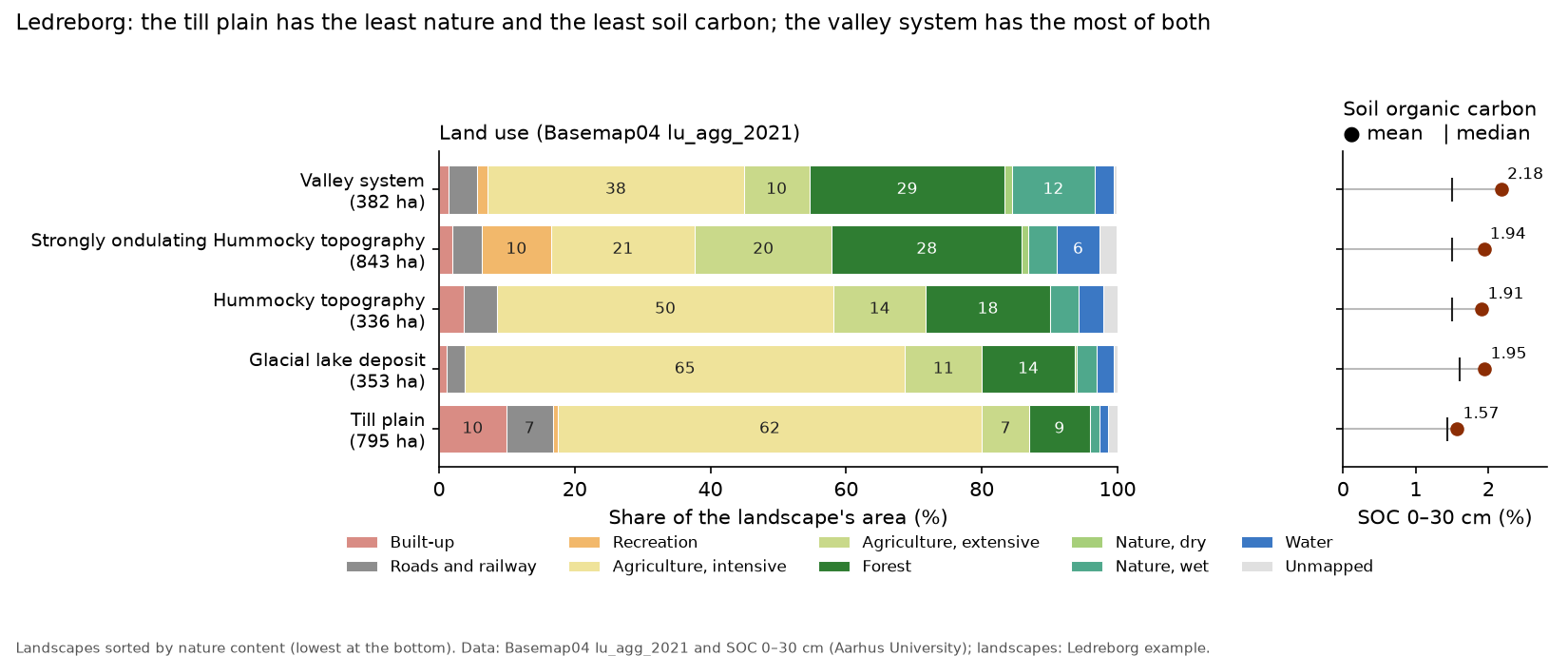
Landscape	Intensive arable	Forest	Wet nature	Mean SOC	Median SOC
Valley system	38 %	29 %	12 %	2.18 %	1.50 %
Glacial lake deposit	65 %	14 %	3 %	1.95 %	1.60 %
Strongly ondulating hummocky topography	21 %	28 %	4 %	1.94 %	1.50 %
Hummocky topography	50 %	18 %	4 %	1.91 %	1.50 %
Till plain	62 %	9 %	1.5 %	1.57 %	1.44 %

Intensive arable includes permanent crops; wet nature includes wet nature with extensive agriculture.

Mean SOC 0–30 cm by land use, within the landscapes: wet nature 6.4 %, wet nature with extensive agriculture 5.0 %, lakes 3.9 % (a model artefact, see below), forest 1.9 %, extensive agriculture 1.7 %, intensive arable 1.5 %.

5. Points for the discussion

• The mean hides where the carbon is. In the valley system the median (1.5 %) is the same as elsewhere; the high mean comes from a small wet area with very high values. Carbon management there is about a few hectares of wet soil, not the whole landscape.
• Land use or landform? Wet nature has high SOC, but wet nature also lies where the soil was always wet. The map shows co-occurrence, not that changing land use would change SOC at the same rate.
• Concentration is not stock. 6 % SOC in a light peat soil and 2 % in a dense clay soil can hold similar amounts of carbon per hectare. A carbon budget needs bulk density and depth.
• Habitat and carbon together. The wet areas that hold the most carbon are also §3 nature and part of the habitat network (Habitat network at Ledreborg (Example)). Taking low-lying arable land out of drainage would serve both; the till plain’s stepping stones would mostly serve biodiversity.
• Modelled values under lakes. The SOC model gives lakes 3.9 %; that is the model’s prediction for a soil that is not there, and such cells should be left out of a careful analysis.

Sources

• Møller, A. B., Nyborg, L., Grogan, K., Druce, D., Svane, S. F., Greve, M. B., Gutierrez, S., Styczen, M., Greve, M. H., Knudsen, L. and Beucher, A. (2025). High-resolution 3D soil texture mapping in Denmark using satellite time series and bare soil composites. Advances in Agronomy 194, 133–. doi:10.1016/bs.agron.2025.07.001
• Basemap04 (lu_agg_2021), DCE – Danish Centre for Environment and Energy, Aarhus University.