Dwelling size by construction period in Copenhagen — Example
A worked case in quantitative place analysis for urban planning, on scale in planning. Data: every dwelling in Københavns Kommune from BBR, October 2026.
Across Copenhagen, dwellings built since 2000 are only slightly larger than those built before 1940: 89 against 86 m² on average. Mapped by kvarter, the two periods show different cities. Mapped at three scales, the same dwellings show three different cities again. The question is simple; the answer depends on the categories, the zones and the classes.
The case runs through the four phases of the SemanticGIS workflow. Each step is a Task with a QGIS Recipe, and the same steps answer other questions about BBR data.
Example data
Everything these examples use, frozen as it was used (BBR and DAR, 24 October 2026), so their numbers can be reproduced without API keys: copenhagen_dwellings_example_data.zip (7 MB), a snapshot package. It holds the 349,743 standing dwellings on their address points as GeoParquet (codes only; addresses and register ids are left out), Copenhagen’s four statistical divisions as a GeoPackage, the BBR code lists that name the codes (codelists/), and snapshot.json and a README with sources and attribution. The same data serve Share of rented dwellings in Copenhagen (Example) and Dwelling size by construction period in Copenhagen (Example).
1. Spatial Intent
Question: has new housing in Copenhagen been built larger or smaller than the old housing stock, and does that differ between parts of the city?
Units of observation: dwellings (BBR units used as dwellings), placed on their entrance’s address point.
Units of presentation: Copenhagen’s statistical divisions: 10 bydele, 67 kvarterer and 400 roder (reference units published with SemanticGIS).
2. Auditing the data
| Variable | BBR field | Choice made | Why |
|---|---|---|---|
| Dwelling | status, use code (anvendelse_kode) | standing dwellings (status 6), use 110–190 except student housing (150) and institutions (160) | 9,958 student rooms and institution dwellings, often 15–20 m², would dominate the means of a few areas |
| Construction period | opfoerelsesaar (the building’s construction year) | before 1940 and 2000 or later | the pre-war stock against the recent; the years between are left out |
| Dwelling size | samlet_areal (total area) | total area | areal_beboelse (residential area) differs for only 1,021 of 349,743 dwellings |
What the data cannot say:
- The construction year belongs to the building. A dwelling in a converted building carries the building’s year: Artillerivej 63 in Ørestad Nord has 141 student rooms dated 1918.
- 3,555 dwellings have no construction year.
- Areas are registered values, reported by owners and municipalities, not measured for this analysis.
3. The Analytical Schema
flowchart LR
  R[Categories from register codes] --> A[Aggregating points to zones]
  Z[Statistical divisions] --> A
  A --> C[Comparable choropleth maps]
  A --> S[Same variable at three scales]
| Task | Recipe | Operator families used |
|---|---|---|
| Categories from register codes (Task) | Categories from register codes (Recipe - QGIS) | Selection, Attribute calculation |
| Aggregating points to zones (Task) | Aggregating points to zones (Recipe - QGIS) | Aggregation, Attribute calculation |
| Comparable choropleth maps (Task) | Comparable choropleth maps (Recipe - QGIS) | — (see Classification for maps) |
The choices in short: mean of samlet_areal per kvarter; at least 20 dwellings per kvarter, otherwise shown grey; the same six classes (under 60 to 120 m² or more, in steps of 15 m²) on both maps.
Settings used
- Data: the example data above:
dwellings.parquet(standing dwellings on their address points, from BBR and DAR; see Share of rented dwellings in Copenhagen (Example) for how they were placed) and the divisionsbydel,kvarter,rodeindivisions.gpkg. The names of the codes are incodelists/. - Categories (Categories from register codes (Recipe - QGIS)):
"opfoerelsesaar" < 1940 AND "anvendelse_kode" NOT IN (150, 160)and"opfoerelsesaar" >= 2000 AND "anvendelse_kode" NOT IN (150, 160): 189,650 and 59,878 dwellings. - Aggregation (Aggregating points to zones (Recipe - QGIS)): Join attributes by location (summary), intersect, field
samlet_areal, count, mean, median. The kvarterer hold all 189,650 pre-1940 dwellings, the bydele 189,649 (one lies just outside the bydel layer). With a minimum of 20 dwellings, 5 and 8 of 67 kvarterer have too few, and 50 and 261 of 400 roder. - Spread and shape (below): Join attributes by location, intersect, one-to-many, adding the kvarter’s
navnto each dwelling; then Statistics by categories onsamlet_areal, grouped bynavn. It returns count, mean, median, standard deviation, minimum, Q1, Q3, maximum and interquartile range per kvarter. The quartile skewness is added with the field calculator:("q3" + "q1" - 2 * "median") / "iqr". - Maps (Comparable choropleth maps (Recipe - QGIS)): Categorized on the expression below, the same style on both maps.
CASE WHEN coalesce("samlet_areal_count", 0) < 20 THEN 'Fewer than 20 dwellings'
     WHEN "samlet_areal_mean" < 60  THEN 'under 60 m²'
     WHEN "samlet_areal_mean" < 75  THEN '60–75 m²'
     WHEN "samlet_areal_mean" < 90  THEN '75–90 m²'
     WHEN "samlet_areal_mean" < 105 THEN '90–105 m²'
     WHEN "samlet_areal_mean" < 120 THEN '105–120 m²'
     ELSE '120 m² or more' END
4. Results
Two periods, one set of classes
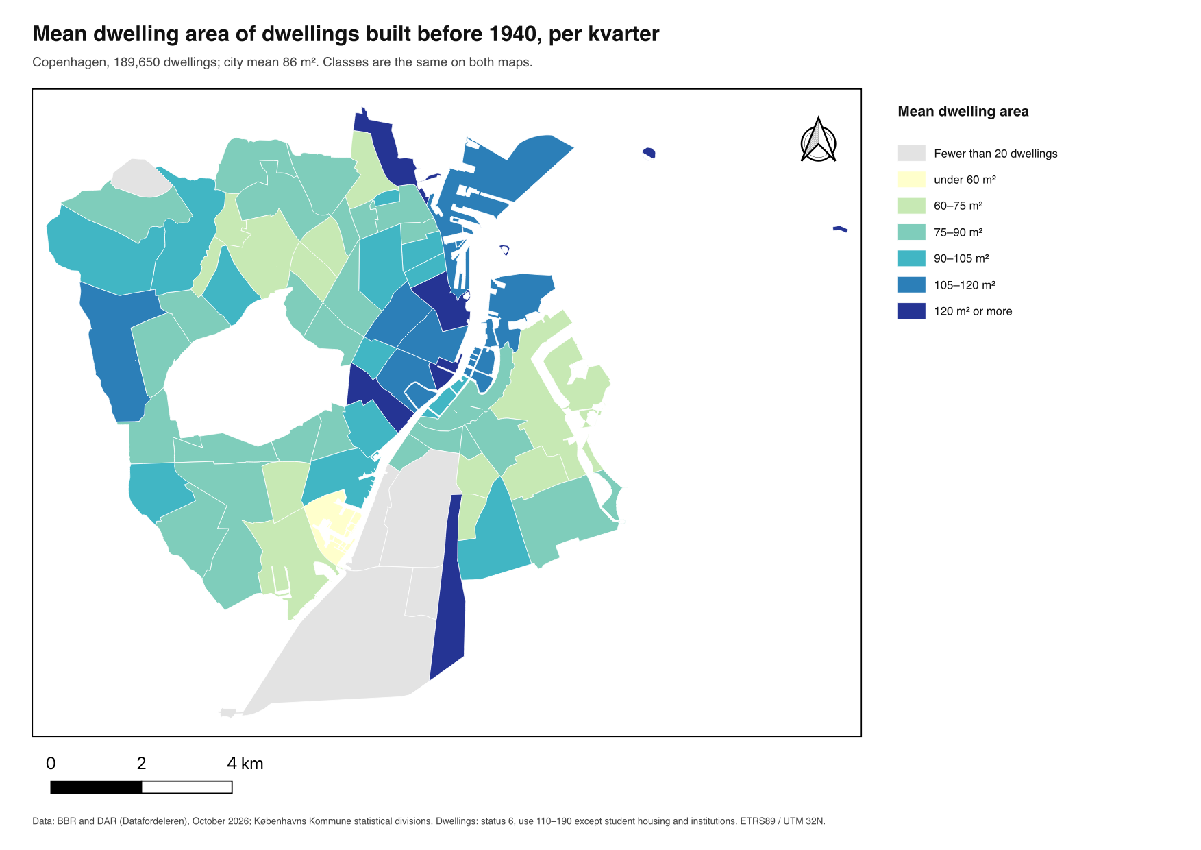
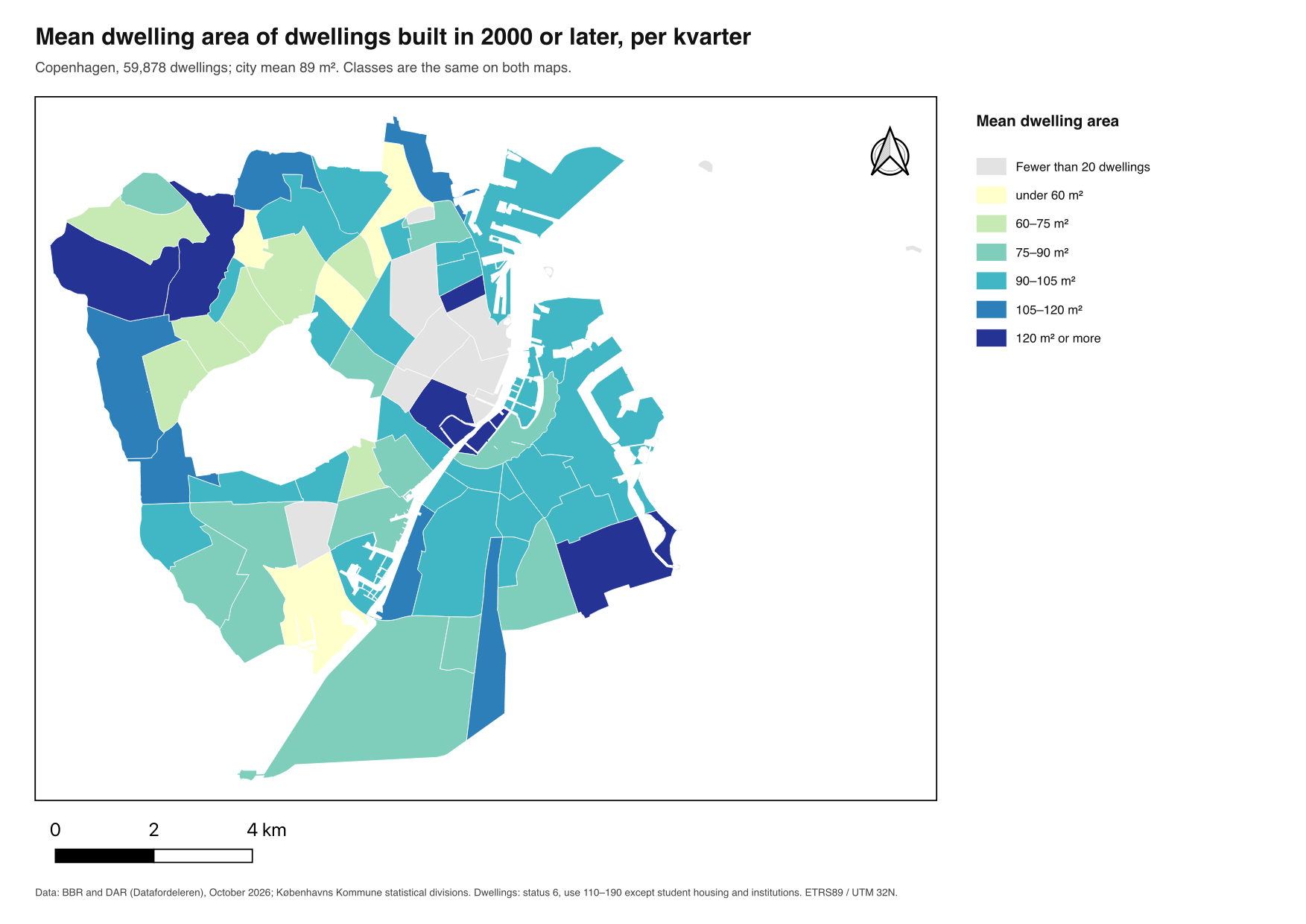
| Built before 1940 | Built 2000 or later | |
|---|---|---|
| Dwellings | 189,650 | 59,878 |
| City mean | 86 m² | 89 m² |
| Kvarterer with at least 20 dwellings | 62 of 67 | 59 of 67 |
| Smallest kvarter means | Holmene 43 m², Bavnehøj 62 m², Urbanplanen 65 m² | Utterslev 43 m², Ny Ryvang 46 m², Lyngbyvej Vest 57 m² |
| Largest kvarter means | Østerbro Nord 135 m², Østerport 135 m², Metropolzonen 136 m² | Villakvartererne 139 m², Christianshavn Neden Vandet 139 m², Husum 153 m² |
Before 1940, the largest dwellings are in Østerbro Nord, Østerport and Metropolzonen, the smallest on Holmene (the former naval base), at Bavnehøj in Sydhavn and in Urbanplanen on Amager. Since 2000, the largest new dwellings are in two outer districts (Husum and the villa districts) and on Christianshavn, the smallest in the north-west and north (Utterslev, Ny Ryvang). Much of the inner city has fewer than 20 new dwellings and is grey. The two city means, 86 and 89 m², hide all of this.
The same dwellings at three scales
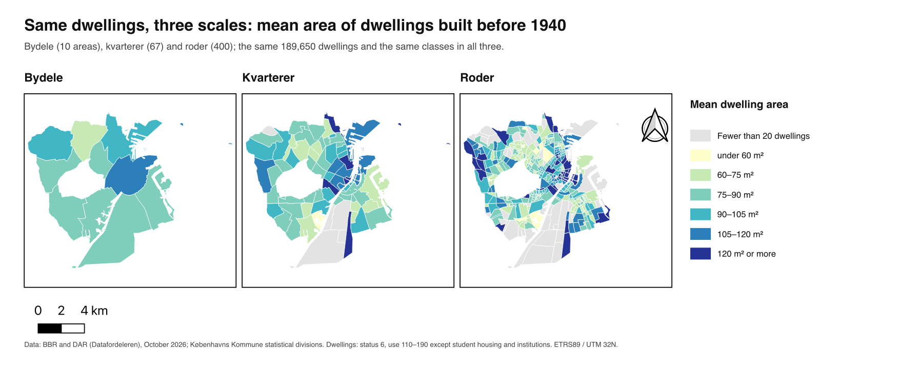
| Zones (pre-1940 dwellings) | Zones with ≥ 20 dwellings | Lowest – highest mean | Standard deviation of the means |
|---|---|---|---|
| Bydele | 10 of 10 | 70 – 111 m² | 10.5 m² |
| Kvarterer | 62 of 67 | 43 – 136 m² | 18.5 m² |
| Roder | 350 of 400 | 43 – 243 m² | 23.9 m² |
For dwellings built since 2000 the effect is stronger still: 261 of the 400 roder have fewer than 20 such dwellings, because new housing is concentrated in a few areas. At rode level, the map of new housing is mostly grey.
Spread and shape within the kvarterer
The maps show one number per kvarter, the mean. Two kvarterer with the same mean can hold dwellings of one size or a mix of very small and very large, and the map cannot tell them apart.
A pragmatic choice of tools. A summary tool returns the statistics it offers per zone, and nothing else: Join attributes by location (summary) gives count, mean, median and a few more. The alternative is two steps: first give each dwelling its zone (Join attributes by location, one-to-many), then summarise by group (the group-by statistics Operator, here Statistics by categories). The joined dwellings remain available, so any statistic can be computed per zone afterwards, the distribution inside one kvarter can be drawn as a histogram, and the dwellings behind an extreme value can be found.
Reading spread and shape from the quartiles. The minimum, Q1, median, Q3 and maximum indicate dispersion and shape without a dedicated tool:
| Compare | Indicates |
|---|---|
| mean − median | skew: positive when a few large dwellings pull the mean up, negative when a few small ones pull it down |
| interquartile range, Q3 − Q1 | the spread of the middle half of the dwellings, unaffected by extreme values |
| Q3 − median against median − Q1 | whether the middle half is symmetric; as one number the quartile skewness, (Q3 + Q1 − 2 · median) / IQR, between −1 and 1 |
| maximum against Q3 | extreme values, to check before they are averaged |
| Kvarter | Built | Dwellings | Mean | Median | Q1 – Q3 | IQR | Maximum |
|---|---|---|---|---|---|---|---|
| Holmene | 2000 or later | 7,271 | 95 m² | 95 m² | 85 – 106 m² | 21 m² | 242 m² |
| Bispebjerg | 2000 or later | 200 | 95 m² | 90 m² | 46 – 131 m² | 85 m² | 254 m² |
| Ny Ryvang | 2000 or later | 118 | 46 m² | 45 m² | 45 – 46 m² | 1 m² | 52 m² |
| Holmen og Refshaleøen | before 1940 | 152 | 112 m² | 52 m² | 37 – 172 m² | 135 m² | 363 m² |
| Frederiksstaden | before 1940 | 3,993 | 113 m² | 94 m² | 63 – 139 m² | 76 m² | 3,519 m² |
- Same mean, different kvarterer. New dwellings in Holmene and Bispebjerg average 95 m² and get the same colour. In Holmene the middle half lies between 85 and 106 m², in Bispebjerg between 46 and 131 m².
- No spread at all. Half of Ny Ryvang’s 118 new dwellings are 45 or 46 m²: almost all of one size, so the mean describes a building type rather than a mix.
- A mean that describes no dwelling. Holmen og Refshaleøen’s pre-1940 dwellings have a mean of 112 m² and a median of 52 m²: many small dwellings and some very large ones. Whether they form two separate groups the quartiles cannot show; a histogram of the kvarter’s joined dwellings can.
- One value moves the standard deviation. In Frederiksstaden one dwelling is registered with 3,519 m². The standard deviation is 117 m², the interquartile range 76 m². A value like that belongs in the audit (section 2) before it goes into any mean.
- The two periods are skewed differently. Before 1940 the mean is above the median in 60 of the 62 kvarterer shown: a stock of mostly small dwellings with a tail of large ones. For dwellings built since 2000 the median is above the mean in 25 of 59. Comparing the two maps of means therefore compares differently shaped distributions, and a map of medians beside each map of means shows where that matters.
5. Points for the discussion
- Scale effect. Smaller zones show more variation: ten bydele look alike, four hundred roder do not. Neither is “the true” picture; each answers a question at its own scale, from city strategy to local plan.
- Zoning effect. Kvarterer and roder are drawn for administration. A grid of the same size, or the same grid moved half a cell, gives other values: the same dwellings, other maps (see Modifiable areal unit problem and Share of rented dwellings in Copenhagen (Example)).
- Small numbers. The minimum count decides which areas get a value. A kvarter with 25 new dwellings and one with 2,500 get the same weight on the map.
- Categories are choices. With student housing included, Ørestad Nord’s pre-1940 dwellings average 17 m² (141 student rooms at Artillerivej 63); without it, the kvarter has too few pre-1940 dwellings to show. A different definition of “dwelling” gives a different map.
- Numbers without context. A mean of 153 m² in Husum and 43 m² in Utterslev raise questions the data cannot answer: which projects, for whom, under which plans? Quantitative place analysis points to where to look; it does not explain what is found.
- Ecological fallacy. A kvarter’s mean does not describe a typical dwelling in it; a mix of very large and very small dwellings gives the same mean as uniform medium ones.
Teaching use
The Recipes give every setting and end with check numbers, so students can follow this case step by step and then apply the same Tasks to their own question and variables.