Share of rented dwellings in Copenhagen — Example

A worked case in aggregating point data to areas, for urban planning. Data: every dwelling in Københavns Kommune from BBR, October 2026. Companion: Dwelling size by construction period in Copenhagen (Example).

Three QGIS tools turn 349,743 dwelling points into maps of districts, and they give the same answer when they are used the same way. What changes the answer is the choice of areas: across 10 districts the share of rented dwellings runs from 65 to 87 %, across 928 cells of 250 m from 0 to 100 %. The data did not change; the map did.

Example data

Everything these examples use, frozen as it was used (BBR and DAR, 24 October 2026), so their numbers can be reproduced without API keys: copenhagen_dwellings_example_data.zip (7 MB), a snapshot package. It holds the 349,743 standing dwellings on their address points as GeoParquet (codes only; addresses and register ids are left out), Copenhagen’s four statistical divisions as a GeoPackage, the BBR code lists that name the codes (codelists/), and snapshot.json and a README with sources and attribution. The same data serve Share of rented dwellings in Copenhagen (Example) and Dwelling size by construction period in Copenhagen (Example).

Why aggregate?

In Denmark almost all statistical data are collected at the address point. Data about buildings and dwellings are registered in BBR at the building’s and the dwelling’s address; socio-economic data describe individuals through their CPR number, and each person is registered at an official address. So the raw material of Danish statistics is points: one per building, dwelling or person.

These points are rarely shown as they are, for two reasons:

• Too much detail hides the pattern. Copenhagen alone has 349,743 dwellings. On a map of points the dense areas become solid blots.
• Points can identify people. A point with an income or a diagnosis attached is a person. Statistics may only be published in a form where no individual can be recognised.

So we aggregate: count, sum or average the points that fall in each of a set of areas, and show the areas instead of the points. The areas can be administrative (bydele, kvarterer, roder) or made for the purpose, such as a grid. Whichever we choose, the result depends on that choice: the Modifiable areal unit problem.

The data and the areas

Layer	What it is	Features
Dwellings (points)	standing dwellings (BBR units with status 6, use 110–190) on their entrance’s address point; see Placing register units on the map (Task)	349,743
Bydele	the city’s districts	10
Lokaludvalg	local council areas	12
Kvarterer	statistical neighbourhoods	67
Roder	the smallest statistical units	400
Grids	squares of 1,000, 500 or 250 m, or hexagons, made with Create grid (Tool - QGIS)	any

The divisions are Copenhagen’s own, the same that Statistikbanken uses, published as reference units. A grid is a set of statistical areas like the roder, drawn by rule instead of by an administration. Everything is in EPSG:25832.

Data files

The dwellings were placed on the map with Placing register units on the map (Recipe - QGIS), from Datafordeleren’s file downloads (TotalDownload, csv, Current), October 2026:

Table	Download	Rows used
BBR_Enhed	BBR, Enhed, municipality 0101	491,935 units
BBR_Bygning	BBR, Bygning, municipality 0101	92,813 buildings
DAR_Adresse	DAR, Adresse (national file)	478,086 on Copenhagen’s house numbers
DAR_Husnummer	DAR, Husnummer (national file), filtered to "kommuneinddeling" = 389103	89,087
DAR_Adressepunkt	DAR, Adressepunkt, municipality 0101	one per house number

8,590 units found no address (all historic, closed or registered in error) and 1,672 no building point; every standing dwelling got an address point. The result is boliger.gpkg; the divisions are in kk_enheder.gpkg, or with the SemanticGIS plugin under Københavns Kommune statistical units.

Preparing the points

1. Keep only standing dwellings (Extract by expression (Tool - QGIS)): "status_kode" = 6 AND "anvendelse_kode" BETWEEN 110 AND 190. 349,743 points: every aggregation below must add up to this number.
2. Turn the category into a 0/1 field (Field calculator (Tool - QGIS)): udlejet = if("udlejning_kode" = 1, 1, 0). The sum of udlejet is the number of rented dwellings, and its mean is the share rented (indicator variable). Across the city the share is 75.5 %, and the mean dwelling is 81.7 m².

Two choices hide in these steps: dwellings marked not in use count as not rented, so they are in the denominator; and each dwelling sits on its entrance’s address point, not its building’s point.

Method 1: Count points in polygon

Count points in polygon (Tool - QGIS) with the bydele as polygons gives one count per bydel; with udlejet as Weight field it gives the number of rented dwellings.

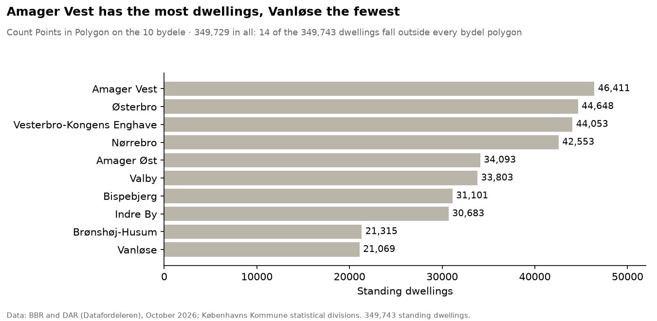
The missing 14 dwellings show why the sum is worth checking: the kvarter layer contains all 349,743, so the two layers’ outer edges do not quite match. The tool gives only a count or a sum, so a share needs two runs and a field calculation.

Method 2: Join attributes by location (summary)

Join attributes by location (summary) (Tool - QGIS) does the whole job in one run: kvarterer as Join to features in, the dwellings as By comparing to, fields samlet_areal and udlejet, summaries count, sum, mean and median. udlejet_mean is the share rented.

Kvarter	Dwellings	Share rented	Mean area (m²)	Median area (m²)
Bryggen Syd	2,584	36 %	113	107
Nordhavn	3,705	41 %	99	99
Jyllingevej Kvarter	5,059	45 %	96	88
Bispebjerg	3,447	91 %	76	68
Tingbjerg	2,613	92 %	75	79
Ny Ryvang	1,901	94 %	69	73

Mean and median tell different stories when a few very large dwellings pull the mean up, as in Bryggen Syd. The long way — give each point its kvarter with Join attributes by location (Tool - QGIS), summarise with Statistics by categories, and join back with Join attributes by field value (Tool - QGIS) — gives exactly the same numbers.

Method 3: density

A count is not a density: a large kvarter has many dwellings partly because it is large.

• Density per area: on the output of method 2, coalesce("udlejet_count", 0) / ($area / 1000000) gives dwellings per km². It runs from 18,568 per km² in Amagerbro vest down to 689 at Grønjordssøen, where the denominator includes large undeveloped areas.
• Kernel density: Heatmap (Tool - QGIS) (radius 500 m, cell 50 m, kernel Quartic, output Raw) spreads each point over a circle and adds the circles up into a raster, with no areas at all. Its radius plays the role the areas played.

Same dwellings, different maps

Averaging the roder’s shares to get a bydel’s share is wrong in eight of ten bydele, and the share rented spreads further the smaller the areas are: see Modifiable areal unit problem for both charts and the rules that follow.